NBeats
Finally got chance to jog down some notes around the N-BEATS paper.
Main contributions
- 1) deep neural architecture: Pure deep learning network without time-series specific componets that performed better than well-established statistical models on reference time-series datasets (e.g. M3, M4, etc.).
- 2) interpretable DL for time series
Algorithm
- Task: Predict the vector of future values (\(\mathbb{y} = [y_{T+1}, y_{T+2}, ..., y_{T+H}]\)) of length H forecast horizon given a length T observed historical series \([y_{1}, y_{2}, ..., y_{T}]\).
- if define a lookback window of length t \(\leq\) T from \(y_T\), the model period can be denoted as \(\mathbb{x} = [y_{T-t+1}, y_{T-t+2}, ..., y_{T}]\)
- the forecasts are \(\hat{\mathbb{y}}\)
- Common evaluation metrics for time-series forecasts are:
- MAPE (mean absolute percentage error): \(\frac{100}{H}\sum_{i=1}^H \frac{\left| y_{T+i}-\hat{y}_{T+i} \right| }{|y_{T+i}|}\) (the errors are scaled by the ground truth)
- SMAPE (symmetric MAPE): \(\frac{200}{H}\sum_{i=1}^H \frac{\left| y_{T+i}-\hat{y}_{T+i} \right| }{|y_{T+i}| + |\hat{y}_{T+i}|}\) (the errors are scaled by the average of forecast and ground truth)
- MASE (mean absolute scaled error): \(\frac{1}{H}\sum_{i=1}^H \frac{\left| y_{T+i}-\hat{y}_{T+i} \right| }{\frac{1}{T+H-m} \sum_{j=m+1}^{T+H}|y_j - y_{j-m}|}\) (the errors are scaled by the average error measured m periods in the past, accounting for seasonality)
- Architecture:

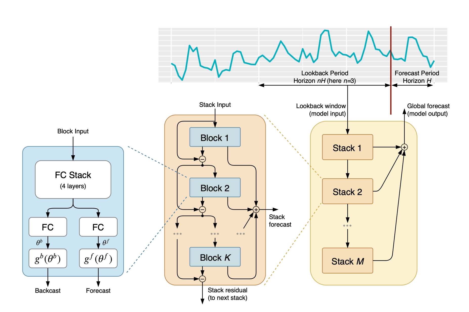
- Basic block: (blue figure) Take 1 Block input vector (\(x_l\)) and output 2 vectors: \(\hat{x_l}\), the backcast (usually with length of 2H - 7H) + \(\hat{y_l}\), the forecast (usually with length of H)
- Block 1’s input is the overall model input (\(x_l\)): lookback values within the defined window (\(x_l\))
- Block 2 - L’s input is the the backcast residual values from the previous layer (\(x_l\) = \(x_{l-1} - \hat{x}_{l-1}\))
- Within the Block, the default algorithm is consist of 4 standard fully-connected (FC) layers with ReLU non-linearity stacking in sequence with 2 linear output layers.
- Doubly residual stacking (orange+yellow figure): An extension from the classic ResNet architecture, e.g. Input vector (x) is added to the output vector (F(x)) before passing to the next stack. The proposed architecture involved the two residual branches (forecast and backcast) as described in above section within each block, and stack the residues between blocks with the following two equations:
- Backcast residual branch, each depending on residues from previous block: \(x_l\) = \(x_{l-1} - \hat{x}_{l-1}\)
- Forecast residual branch, summation of forecasts by all blocks within a stack: \(\hat{y} = \sum_l \hat{y}_l\)
- Both equations are repeated as the same architecture across stacks and the final forecasts are the summation of \(\hat{y}\)
- Aboves were notes over a generic model setup without time-series specific knowledge on none-linear trend or seasonality (a.k.a the assumptions on \(g_b\) and \(g_f\) specified in the cartoon figure were linear). That says, with additional assumptions made on the two equations across blocks/stacks, we’re also able to incorporate TS-specific assumptions in for tuning.
Helpful videos & blogs:
- ResNets and Why ResNets work by DeepLearningAI
- An Overview of ResNet and its Variants